This post discusses lexicon-based sentiment classifiers, its advantages and limitations, including an implementation, the Sentlex.py library, using Python and NLTK.
A sentiment classifier takes a piece of plan text as input, and makes a classification decision on whether its contents are positive or negative. For simplicity, lets assume that input text is known a priori to be opinionated (which we could obtain by filtering input text through another classifier that detects opinionated text from neutral ones).
We want to explore lexicon-based approaches to sentiment classification. These methods use a language resource - a sentiment lexicon - that associates words and expressions to an opinion polarity - usually a numeric score, representing common knowledge about this word's opinion.
Why use sentiment lexicons? One advantage of this method is that, unlike supervised learning approaches, it can be applied to text with no training data required, making it an interesting alternative for cases where training data is non existent or when we're dealing with data from multiple domains. In particular, it is an interesting strategy (although not the only one) for dealing with domain dependence problems seen on supervised learning sentiment classification methods.
Lets take a look at sentiment lexicons in sentlex:
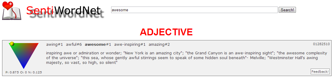
The SWN3Lexicon() class is a subclass of ResourceLexicon(), which does two things upon instantiation: reads a specific language resource into memory (in this case SentiWordNet v3.0), and compiles word frequency data based on the frequency distribution of lexicon words in NLTK's Brown corpus.
Using this class we can query a word when used as a specific part of speech (adjective, verb, noun and adverb) using getadjecvive(), getverb() and so on. These methods return a tuple of numeric values (positive, negative) indicating word polarity known to the lexicon. Another simplification implemented here applies when words carry multiple senses: the opinion of each of those is averaged out to obtain the output tuple - ie. other than separating words by part of speech, no word sense disambiguation takes place.
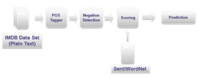
How to classify test with a sentiment lexicon? A simple strategy is to scan a document counting the words found in the lexicon, and make a classification decision based on the total counts for positive and negative words found. SentiWordNet contains words part-of-speech information, so it makes sense to perform some pre-processing on input text: we'll use NLTK's part-of-speech tagger to find out what part-of-speech to query in the lexicon for each word found.
Lets begin by looking at what the sentiment classifier does using sentutil:
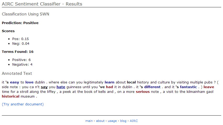
The output of this script is a tuple (positive, negative) containing the overall positive and negative sentiment for the document (in the above example, we classify the document as positive). It also generates an annotated version of the input document with part of speech tags and additional tags indicating sentiment scores for each word.
The heart of the operation are the subclasses implementing DocSentiScore, and in particular the implementation of classify_document() method. To classify an input document, we instantiate this class with specific parameters for how the algorithm should work, and a sentiment lexicon. DocSentiScore class takes in a Lexicon object to perform classification, so it is easy for example, to swap lexicons and evaluate its effect.
The parameters here vary with implementation, In the example below we configure BasicDocSentiScore with SentiWordNet lexicon, scanning for adjectives and verbs, and scoring all occurrences of a given word.
At the end of running classify_document, the result_data dictionary is populated with classification outcome, the annotated document and other information extracted from the algorithm. Most of sentiment data in this example comes from adjective words (tagged with /JJ: "great", "helpful", etc). This is perhaps unsurprising but illustrates how part-of-speech tagging can help filter good signals for sentiment classification. Plus, this is a good fit for SentiWordNet which is also has its contents divided into parts of speech.
In the next post, I'll discuss negation detection and score adjustments in more detail, and use that to refine our classifier.
Some references and links:
A sentiment classifier takes a piece of plan text as input, and makes a classification decision on whether its contents are positive or negative. For simplicity, lets assume that input text is known a priori to be opinionated (which we could obtain by filtering input text through another classifier that detects opinionated text from neutral ones).
We want to explore lexicon-based approaches to sentiment classification. These methods use a language resource - a sentiment lexicon - that associates words and expressions to an opinion polarity - usually a numeric score, representing common knowledge about this word's opinion.
Why use sentiment lexicons? One advantage of this method is that, unlike supervised learning approaches, it can be applied to text with no training data required, making it an interesting alternative for cases where training data is non existent or when we're dealing with data from multiple domains. In particular, it is an interesting strategy (although not the only one) for dealing with domain dependence problems seen on supervised learning sentiment classification methods.
Lets take a look at sentiment lexicons in sentlex:
The SWN3Lexicon() class is a subclass of ResourceLexicon(), which does two things upon instantiation: reads a specific language resource into memory (in this case SentiWordNet v3.0), and compiles word frequency data based on the frequency distribution of lexicon words in NLTK's Brown corpus.
Using this class we can query a word when used as a specific part of speech (adjective, verb, noun and adverb) using getadjecvive(), getverb() and so on. These methods return a tuple of numeric values (positive, negative) indicating word polarity known to the lexicon. Another simplification implemented here applies when words carry multiple senses: the opinion of each of those is averaged out to obtain the output tuple - ie. other than separating words by part of speech, no word sense disambiguation takes place.
How to classify test with a sentiment lexicon? A simple strategy is to scan a document counting the words found in the lexicon, and make a classification decision based on the total counts for positive and negative words found. SentiWordNet contains words part-of-speech information, so it makes sense to perform some pre-processing on input text: we'll use NLTK's part-of-speech tagger to find out what part-of-speech to query in the lexicon for each word found.
Lets begin by looking at what the sentiment classifier does using sentutil:
The output of this script is a tuple (positive, negative) containing the overall positive and negative sentiment for the document (in the above example, we classify the document as positive). It also generates an annotated version of the input document with part of speech tags and additional tags indicating sentiment scores for each word.
The heart of the operation are the subclasses implementing DocSentiScore, and in particular the implementation of classify_document() method. To classify an input document, we instantiate this class with specific parameters for how the algorithm should work, and a sentiment lexicon. DocSentiScore class takes in a Lexicon object to perform classification, so it is easy for example, to swap lexicons and evaluate its effect.
The parameters here vary with implementation, In the example below we configure BasicDocSentiScore with SentiWordNet lexicon, scanning for adjectives and verbs, and scoring all occurrences of a given word.
At the end of running classify_document, the result_data dictionary is populated with classification outcome, the annotated document and other information extracted from the algorithm. Most of sentiment data in this example comes from adjective words (tagged with /JJ: "great", "helpful", etc). This is perhaps unsurprising but illustrates how part-of-speech tagging can help filter good signals for sentiment classification. Plus, this is a good fit for SentiWordNet which is also has its contents divided into parts of speech.
In the next post, I'll discuss negation detection and score adjustments in more detail, and use that to refine our classifier.
Some references and links:
- This paper from Taboada et al explores Sentiment Classification using lexicons and discusses algorithm variations motivated by negated sentences and intensifiers.
- The code for sentlex is on github under github.com/bohana/sentlex
- The DIT Sentiment Analyser runs an implementation of the libraries above.